Moving on from fluids and oceans, I decided to try my hand at Pyro FX, since this was going to be a section of my final output. Some initial teething problems arose when it came to finding learning resources for Pyro FX in Houdini, whereas previously I had mainly been utilising tutorials available on Pluralsight, I found that the Pyro tutorials available there were well beyond my current skill level within the software. The tutorial went into some depth regarding vector operators, something which I am totally unfamiliar with as well as some scripting, while I usually enjoy a challenge when it comes to learning new software skills, it became very apparent that I was out of my depth.

After discussing the issue with my tutor, we deliberated whether it would be best to utilise this learning resource while stating my ignorance on the subject or not, while he did encourage me to follow along with the video, I did not think it very useful to building my skills, since I wouldn’t actually be learning the necessary methods, but rather just copying the work. I have made a mental note of this set of tutorials however, and will be revisiting them once I feel more comfortable with Houdini.

After some hunting around the internet, I found that the most useful resource available to me regarding Pyro FX was in fact SideFXs own documentation which was available from the user guide within the software itself, after briefly reading through their own explanation of the Pyro FX tools, I began to grasp how to control them.

So when creating a flame for example, a series of nodes is created with the DOP network, much like what occurs when creating FLIP objects, the key difference being the solvers created and the parameters available within them. Unlike FLIP, attached to the Pyro solver is a resize container node, which controls the bounding box which initially surrounds the fire simulation, this is a very important node when creating Pyro and optimizing the scene. The bounding box changes dynamically depending on the size of the fire simulation, but will limit itself based on upper and lower bound parameters, for my own purposes, I found that turning off the ‘clamp to maximum bounds’ attribute suited my purposes better, so as not to cut off any part of my simulation without having to fiddle around with two seperate values. This sort of thing would definitely be more important when working with a power intensive scene, but my scenes were relatively quick to render and simulate, so turning off the clamp did not affect these times too much.

The nodes created upon using the Pyro FX tools.

Also when creating a Pyro sim there are two important values when it comes to the generation of fire or smoke, these values are Fuel and Temperature, Fuel controls where the pyro sim births from, whilst temperature is the value which tells the fuel when to burn, so where fuel exists and temperature is above a certain point, burn is created. Additionally on the fuel source, much like a Flip source, noise can be added to create more turbulence from it’s origin, like Flip this creates a more photoreal, natural look when it comes to the burn.

These are my initial test renders of both fire and smoke, while the quality is not the highest, I think these show off what is possible with Pyro FX in a relatively short amount of time. I will continue to work and experiment with Pyro leading into my final output.

Evaluating these renders and gathering some feedback, the fire was of a very low resolution and it’s interaction and burn was quite uninteresting, to improve this I would most likely change the source object which the flames emit from, as well as changing the various attributes in the Pyro solver to create a more turbulent flame with more character. The smoke on the other hand, while quite satisfying to look at, and of a relatively high quality, looks quite alien, in that it appears like the smoke is in a vacuum, since there is very little dissipation. But for an initial set of test renders, both have displayed to me what is possible with Pyro FX and how I should move forward and improve my skills in this area.

Moving onto the next steps of my project I wanted to experiment further with fluids, more specifically I wanted to replicate some of what I had seen of Dynamic Oceans in a few showreels. To undertake this I utilised the ‘Intro to Dynamic Oceans’ tutorial on Pluralsight. One problem I did run in to whilst making notes on this series of videos, was that once again, it was using an older version of Houdini, which had a completely different set of shelf tools for oceans, as well as a vastly different node layout when using the tools. Luckily, SideFX has a very thorough user guide, which helped me get to grips with some of the changes made in version 16. The tutorials themselves covered most, but not all of the tools available under the oceans tab, going in to a good amount of detail of the parameters which affect the simulations, as well as how to edit the materials applied when rendering. Overall, a very good set of tutorials, which enabled me to go forward and produce a good set of experiments and tests.

Aims

• Get to grips with the ocean tools and produce test renders
• Time my renders to enable me to plan ahead for my final output
• Evaluate my tests and gather feedback from my peers

Prior to undertaking these experiments, I was under the impression that creating an ocean in Houdini would operate very simarlily to creating a FLIP tank, consisting of volumes and particles. However, to my surprise, when using the ocean shelf tool, no DOP network is created, this is because there are actually no dynamics to create. An ocean in Houdini is simulated by first creating a grid, the points of which are then deformed and moved at random to emulate waves.

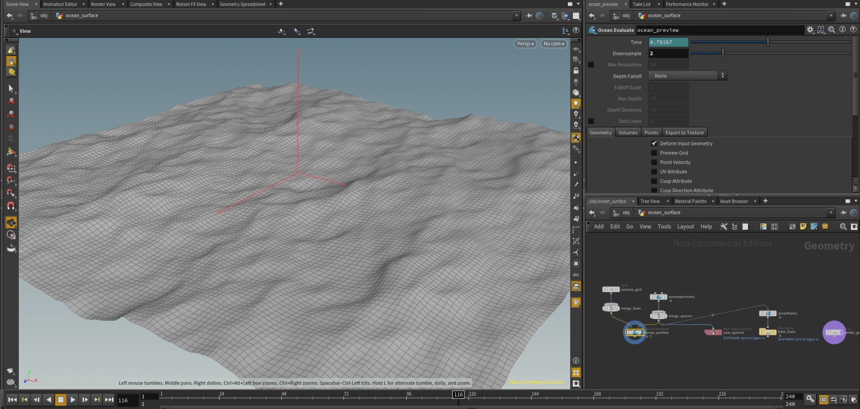
An ocean grid as it appears in the viewport.

The ocean spectrum node under the ocean_surface container is probably the most important node when it comes to controlling the appearance of the simulation, from here you can first control the size and resolution of the grid, the ‘Resolution Exponent’ controls how much detail is in the initial grid, the higher the value of this parameter will obviously create a much more detailed ocean surface. This parameter should also be directly tied to the number of columns and rows in the initial grid, through trial and error it was discovered that the exact value of rows and columns should be 2^ of the resolution exponent, through simply using relative references.

It’s important to note that after doing this I experienced a much slower playback in the viewport, a quick and easy way of remedying this was to use the ‘Downsampling’ parameter under the Ocean Evaluate node, at it’s default the value is a downsample of 2, basically this means that a resolution exponent value of 9 with a downsampling value of 2 will result in the viewport showing a resolution exponent of 7. Raising the downsampling will result in much faster performance in the viewport, without affecting the resolution when it comes to rendering.

Going deeper into the parameters in the ocean spectrum node, the depth value affects the uniformity of small and larger waves within the ocean, deeper oceans have a strong dispersion relationship, meaning larger, low frequency waves will move faster than smaller waves, a low value in the parameter will make both sizes of waves more uniform.

Another interesting feature here is ‘Loop Over Time’, this is essentially what it says on the tin, this can cause your ocean to loop perfectly, setting your Loop period to the length of your scene will mean that there will be no noticeable ‘cut’ between the last and first frame. This is an incredibly useful feature, in an example, if you wanted an ocean in the background of a scene, you can effectively have it loop infinitely whilst only having to actually render around 10 seconds of simulation, which would obviously save a lot of time rendering.

The speed parameter, suprisingly does not actually affect the speed of the waves, instead it controls the rise and fall of the ocean, higher values here will create larger, low frequency waves. This parameter works in tandem with another parameter ‘Scale’ which affects the size of all waves in the scene, large and small.

Directional bias affects how much individual waves will stick to the direction parameter, a high value here will make all waves more uniform in direction, so when creating my ocean I thought it a good idea to leave this value relatively low, as having completely uniform waves would most likely look quite unrealistic.

‘Chop’ affects how sharp the crest of a wave will be, and also works in tandem with the size & speed parameters, a mismatch of all of these values together can create quite a messy looking grid, as some crests will intersect into eachother.

Lastly for the ocean spectrum, is the minimum wave length, which sets the minimum size of all waves in the scene, any waves that are smaller than this value will be smoothed out of the mesh, when creating a calm, placid body of water I imagine this would be quite a useful tool, but for the purpose of a turbulent, choppy ocean, I decided to leave this value at 0.

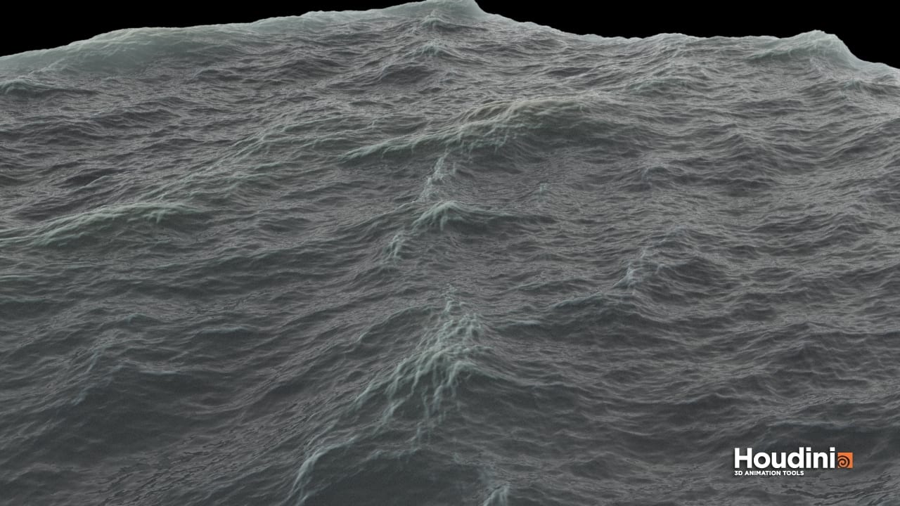
After playing around with these values for a while, I decided to attempt to render out my ocean to get a nice proof of concept as to what to improve and change for my final output. The rendering process itself was initially quite troubling, as when I first attempted a render my ocean came out as a flat grid with no displacement map or texture. Following a tutorial didn’t really provide any help with this, since most of them were using different versions of Houdini. After some experiementing and troubleshooting I found that I had to bake out my displacement maps under the ROP output driver under the ocean_surface node. Once I had done this, I was once again surprised, it was very, very slow. To render one frame of my ocean at 1280 x 720 took 20 minutes. After some quick maths, I decided that it was probably for the best that I not attempt to a full render of 240 frames, since my best estimate on render time would be around 3 days. Further steps from this will most likely lead me to using one of the university lab computers to complete this render, as leaving my PC out of commission for that amount of time wouldn’t be very productive.

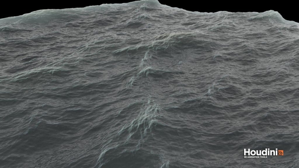
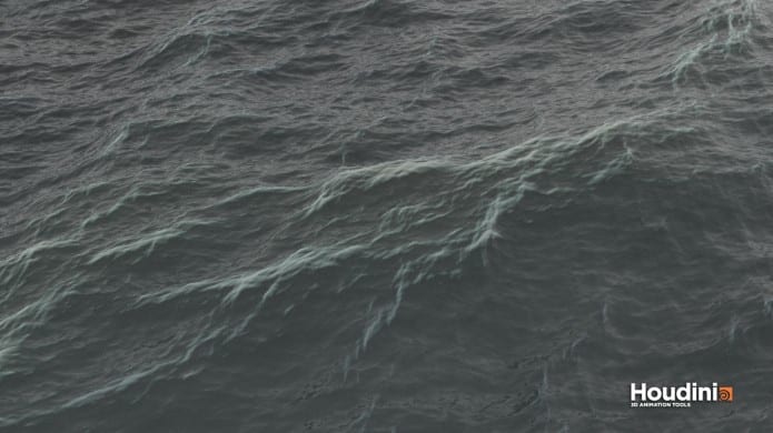
A frame of my ocean.

Evaluating my render, there are definitely some things I would improve. Mainly I want to further play around with the materials of the surface of the ocean and change the color ramps within, definitely increasing the blue values of the deeper sections. Secondly I would also change the displacement values of the foam and crests to make them more apparent, whilst it is a nice subtle effect currently, I really want to emulate realism in this scene, most likely I’ll try to accomplish this by using a lot of reference images to perfect the look. Overall, a decent first attempt at making an ocean, while the render times are certainly a hurdle to overcome, I believe myself to be making good progress in this area.

Continuing on my progress with the tuorials featured on Pluralsight, I moved onto Fluids. The set of tutorials went over some of the basics of the Fluid shelf tools, and explained in some detail exactly what a fluid in Houdini consisted of, as well as how to manipulate them using various methods. On top of this the tutorial briefly covered how to properly optimise fluid simulations, something which became very apparent early on when working with large bodies of water such as FLIP tanks, while my PC is quite high-spec, some of the simulation experiments I conducted during this week slowed my machine down to a crawl, some of which elapsed well over 2 hours just to simulate, which I will go into more detail further into this post. Overall the tutorials were very helpful is gaining a basic understanding of fluids in Houdini and did a great job of maintaining my interest throughout.

Aims

• Learn the basics of fluids in Houdini
• Produce test simulations and renders of my experiments
• Time my simulations and renders to better plan ahead to my final outputs

FLIP Fluids are the standard fluids that I will be working with throughout my time with Houdini, FLIP stands for Fluid Implicit Particle, the reason for this title is that the FLIP system is a hybrid of older methods for producing fluids in Houdini. Before FLIP, fluids were either rendered using volume or particles, the problem with these methods were twofold, volume was an accurate method for producing fluids, but used cumbersome techniques when producing the data for their behaviour (Similar to the method of volume collision detection mentioned in my previous blog post), this resulted in very slow simulation times. And particle fluids were erratic in their behaviour, and could result in unruly simulations. FLIP being the hybrid, takes both of these methods and uses them in tandem with eachother, resulting in an accurate but still somewhat effecient method of calculating fluids.

Upon creating a fluid from a piece of geometry, a large bounding box will surround the particles, this represents the limit of which the fluid can exist within the scene, the use of this being that a clear cutoff point can be created, so when parts of the fluid move out of the viewport, they no longer need to be calculated and make the simulation more efficient.

Looking at the node view, when creating a fluid two nodes are created at the object level, the fluid and the fluid interior, these two nodes mainly effect the appearance of the fluid when rendering out, whilst the tutorials did not go into any detail regarding this, I will have to make a mental note to research how to apply shaders to my fluids, as when I am creating my final outputs, keeping the default shader on my simulations will not result in a realistic look.

Speaking of realism, an important note I made when experimenting with fluids was that not applying any forces other than gravity to my fluids resulted in a very unrealistic look, as all the particles were sticking to the same velocity and direction. An easy method of combatting this was to add turbulence and randomness to the fluids, I achieved this using the ‘Curl noise’ and ‘Vortex’ options within the fluid source node. This resulted in the fluid twisting from the vortex and added some randomness to the initial velocity of the particles with the curl noise option, making my fluid look similar to water ejecting from a faucet.

For this simulation I wanted to do a quick test on my simulation time, according to the fluid output node, at it’s most dense point there were 50,000 particles which made up my fluid. For a 240 frame simulation of a fluid emitter, with both vortex and curl noise added, the simulation took 4 minutes and 30 seconds, overall a good time for developing the look of the fluid, but if I were to render I would obviously up the amount of particles significantly.

Next I moved onto FLIP tanks, unlike fluid emitters, the FLIP tank on its own consists of a constant number of particles and does not move outside of it’s predefined area. I noticed some recent changes to the FLIP tank when researching into the latest version of Houdini, now there is a feature call ‘Narrow Band’ when creating a tank, basically this simulates only the active parts of the tank, leaving any particles under the surface that don’t move unrendered, supposedly this saves on computing power but a quick test of my machine gave a difference of 1 second in simulation time. While it did not make a difference in my FLIP tank simulation, I imagine that a tank with a lower particle separation would benefit greatly in simulation time.

Example of the effects of narrow band.

Below I have embedded a quick render of my flip tank simulation, I added a POP wind node to the DOP network to simulate the waves of the ocean, and using one point of the boat to interact with the motion. While the boats reaction to the water looks quite unnatural, the fluid itself looks somewhat realistic. To improve on this I would first change the motion of the boat, perhaps by inserting some keyframes to smooth out the animation, and secondly I would lower my particle separation to create a more realistic looking fluid.

Simulation Time – 4 minutes 7 seconds

Render Time – 1 hour 32 minutes

Moving on to some further work in Houdini, I wanted to get a better grasp of collisions and dynamics before I moved on to particles, to accomplish these goals I continued to progress through the Houdini Core Skills tutorials featured on Pluralsight. The tutorials themselves covered a broad overall view of how particles and collisions work, again mainly sticking to the shelf tools available within Houdini, but also delving somewhat into VEX expressions without overwhelming the viewer. Topics covered ranged from how particles and collisions work in tandem, the birth attribute and sprites. Overall, these set of tutorials were very helpful on improving my understanding of how each node in the DOP network affects the sim, as well as giving me a good amount of knowledge in how to approach my final sims.

Aims

• Gain a better understanding of how collisions are calculated within Houdini
• Further test and play around with dynamic operators and how they can affect a sim
• Learn the basics of particle operators and some VEX expressions

The particle tools within Houdini, like most tools are either located in the shelf or within the tab menu of the node view. Using the source particle emitter on a piece of geometry will cause all parts of that geometry to emit particles, without any other forces applied to this other than the gravity node which is automatically added, the particles will fall straight down at a constant rate seemily infinitely. To further control how these particles behave, it requires jumping into the DOP network and playing around with some settings. The most important of these settings is under the POP source (Where the particles will emit from), from here you can access the Birth tab, which can control how many particles are emitted per frame and how long these particles will stay in the scene

For optimisation in the simulation, the life expectancy value can be quite important as well, this value controls how long a particle will remain in the scene before it dies. The default value for this is 100 and is measured in seconds, not frames, so a life expectancy value of 1 at 24fps will mean that once a particle reaches the 24th frame of the sim, it will cease to exist. On top of this there is the life variance value, which adds seconds in the positive and negative to randomly assigned particles, the purpose of this being that it creates a more natural cut off point for particles, whereas without it there will be a very abrupt end to the particles emitted. A random seed can also be added to the Life Variance value, resulting in differrent values being applied to the particles.

Particles and the values applied to them are also affected by the framerate of the scene, for example, an emitter with a birth rate of 5000 will generate more particles at 24fps than a scene set at 30fps.

After some experimentation with these values, as well as using the POP velocity tools, I used some geometry provided in the tutorials excersise files to create a basic effect of firing a fire extinguisher, and a space shuttle re-entering the earth’s atmosphere. Both of these effects were created relatively simply, for the fire extinguisher, I had emitted the particles from the nozzle part of the geometry by creating a group node for the selected faces and directing the POP source node to that node, then adding some values to the initial velocity of the particles as well as some variance to these values to create a more natural flow of particles. And for the space shuttle, the particles were emitted from the base of the craft, turning off gravity and then adding a POP wind node into the DOP network so that the particles flew upwards and interacted with the rest of the geometry.

Onto the next set of tutorials, which were relatively short, these covered some of the basics of dynamics which I already had a relatively good understanding of, but went into some greater detail regarding collisions and exactly how they were calculated within Houdini.

Dynamics can be viewed simply as another toolset for animation, which can be a more time effective and realistic method for animation over keyframes, animated a box falling onto a plane can take a long time to animate by hand when aiming for realism, but with dynamics and the shelf tools, can be a relatively simple process with good results.

Diving into the node view in some greater detail, when applying rigid body dynamics or any other set of dynamics to a piece of geometry will create an Auto DOP network which works like a river of data, first the object source node which states where in the node view the geometry will be pulled from, moving onto a merge nodes, which are simply there to filter and combine any nodes to keep the view clean. This then moves onto the most important part of the DOP network, which is the solver, a solver is basically a ruleset which any geometry connected to it must conform to, it contains what constitutes most of a simulation.

Regarding collisions, the Auto DOP network uses collision data to optimise the scene, so without looking at the collisions of a RBD object, the simulation may not represent true to life collisions, which can result in clipping and other oddities when interacting with other RBD objects.

Collision geometry can be calculated in multiple ways, using the RBD solver, collisions can either be calculated using volumes or surfaces. Whilst volume can be a faster method of calculating collision data when working with simpler objects, it gets significantly less accurate using a low amount of divisions. The way this works is that when using the colume for collisions is that Houdini takes a box and places it to encompass the object and the amount of divisions within that box determines how many times the box is divided in the X Y and Z directions. So when working with more complex geometry, a low number of volume divisions will result in an inaccurate set of collision data, whereas a high number of divisions will require significantly more computational power, as this method also analyses spaces within the box with no geometry.

An example of volume collision detection.

Surface collision detection on the other hand can either usse the edges or points of a piece of geometry to collect data, which results in an accurate representation of collisions, without having to calculate any empty space, and purely sticks to the geometry, when working with complex objects, this can be a faster and more efficient method of gathering collision data.

An example of surface collision detection.

Next Steps

• Utilise my knowledge of collisions and particles to produce a few experimental simulations
• Begin to learn about fluids within Houdini