Moving on to some further work in Houdini, I wanted to get a better grasp of collisions and dynamics before I moved on to particles, to accomplish these goals I continued to progress through the Houdini Core Skills tutorials featured on Pluralsight. The tutorials themselves covered a broad overall view of how particles and collisions work, again mainly sticking to the shelf tools available within Houdini, but also delving somewhat into VEX expressions without overwhelming the viewer. Topics covered ranged from how particles and collisions work in tandem, the birth attribute and sprites. Overall, these set of tutorials were very helpful on improving my understanding of how each node in the DOP network affects the sim, as well as giving me a good amount of knowledge in how to approach my final sims.
Aims
- Gain a better understanding of how collisions are calculated within Houdini
- Further test and play around with dynamic operators and how they can affect a sim
- Learn the basics of particle operators and some VEX expressions
The particle tools within Houdini, like most tools are either located in the shelf or within the tab menu of the node view. Using the source particle emitter on a piece of geometry will cause all parts of that geometry to emit particles, without any other forces applied to this other than the gravity node which is automatically added, the particles will fall straight down at a constant rate seemily infinitely. To further control how these particles behave, it requires jumping into the DOP network and playing around with some settings. The most important of these settings is under the POP source (Where the particles will emit from), from here you can access the Birth tab, which can control how many particles are emitted per frame and how long these particles will stay in the scene
For optimisation in the simulation, the life expectancy value can be quite important as well, this value controls how long a particle will remain in the scene before it dies. The default value for this is 100 and is measured in seconds, not frames, so a life expectancy value of 1 at 24fps will mean that once a particle reaches the 24th frame of the sim, it will cease to exist. On top of this there is the life variance value, which adds seconds in the positive and negative to randomly assigned particles, the purpose of this being that it creates a more natural cut off point for particles, whereas without it there will be a very abrupt end to the particles emitted. A random seed can also be added to the Life Variance value, resulting in differrent values being applied to the particles.
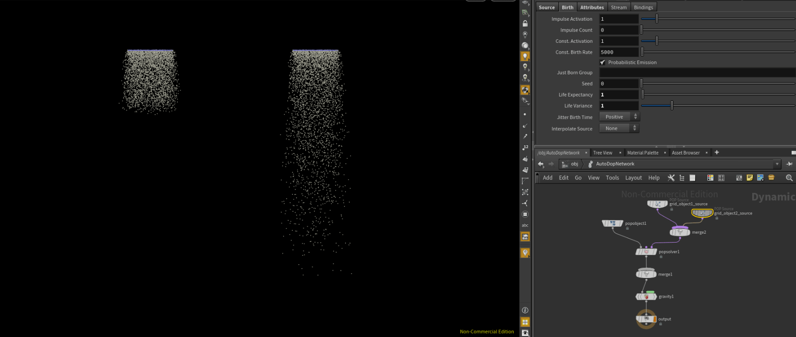
Particles and the values applied to them are also affected by the framerate of the scene, for example, an emitter with a birth rate of 5000 will generate more particles at 24fps than a scene set at 30fps.
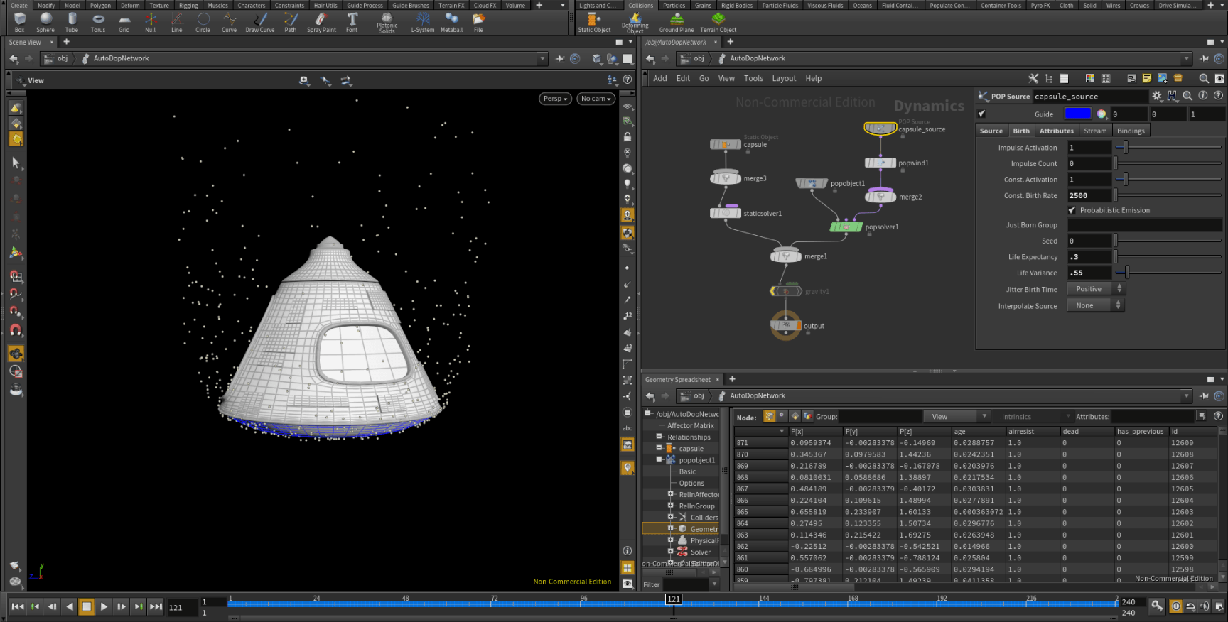
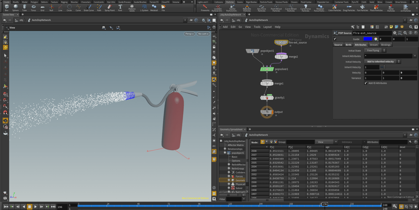
After some experimentation with these values, as well as using the POP velocity tools, I used some geometry provided in the tutorials excersise files to create a basic effect of firing a fire extinguisher, and a space shuttle re-entering the earth’s atmosphere. Both of these effects were created relatively simply, for the fire extinguisher, I had emitted the particles from the nozzle part of the geometry by creating a group node for the selected faces and directing the POP source node to that node, then adding some values to the initial velocity of the particles as well as some variance to these values to create a more natural flow of particles. And for the space shuttle, the particles were emitted from the base of the craft, turning off gravity and then adding a POP wind node into the DOP network so that the particles flew upwards and interacted with the rest of the geometry.
Onto the next set of tutorials, which were relatively short, these covered some of the basics of dynamics which I already had a relatively good understanding of, but went into some greater detail regarding collisions and exactly how they were calculated within Houdini.
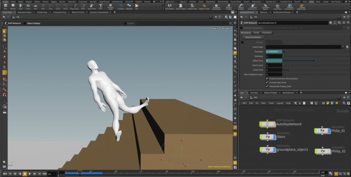
Dynamics can be viewed simply as another toolset for animation, which can be a more time effective and realistic method for animation over keyframes, animated a box falling onto a plane can take a long time to animate by hand when aiming for realism, but with dynamics and the shelf tools, can be a relatively simple process with good results.
Diving into the node view in some greater detail, when applying rigid body dynamics or any other set of dynamics to a piece of geometry will create an Auto DOP network which works like a river of data, first the object source node which states where in the node view the geometry will be pulled from, moving onto a merge nodes, which are simply there to filter and combine any nodes to keep the view clean. This then moves onto the most important part of the DOP network, which is the solver, a solver is basically a ruleset which any geometry connected to it must conform to, it contains what constitutes most of a simulation.
Regarding collisions, the Auto DOP network uses collision data to optimise the scene, so without looking at the collisions of a RBD object, the simulation may not represent true to life collisions, which can result in clipping and other oddities when interacting with other RBD objects.
Collision geometry can be calculated in multiple ways, using the RBD solver, collisions can either be calculated using volumes or surfaces. Whilst volume can be a faster method of calculating collision data when working with simpler objects, it gets significantly less accurate using a low amount of divisions. The way this works is that when using the colume for collisions is that Houdini takes a box and places it to encompass the object and the amount of divisions within that box determines how many times the box is divided in the X Y and Z directions. So when working with more complex geometry, a low number of volume divisions will result in an inaccurate set of collision data, whereas a high number of divisions will require significantly more computational power, as this method also analyses spaces within the box with no geometry.
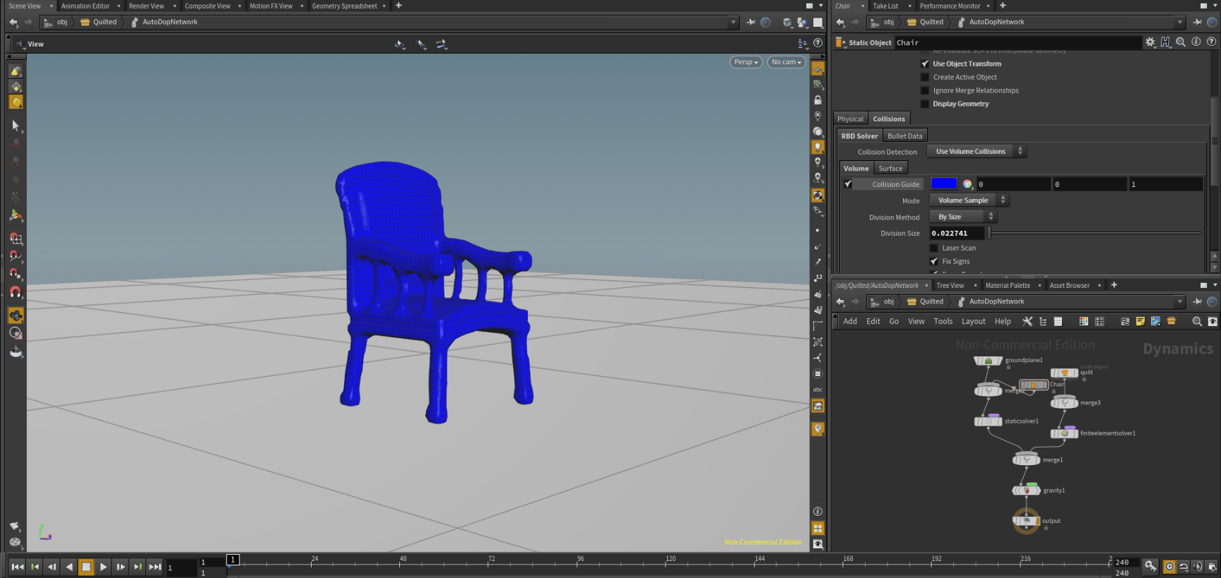
An example of volume collision detection.
Surface collision detection on the other hand can either usse the edges or points of a piece of geometry to collect data, which results in an accurate representation of collisions, without having to calculate any empty space, and purely sticks to the geometry, when working with complex objects, this can be a faster and more efficient method of gathering collision data.
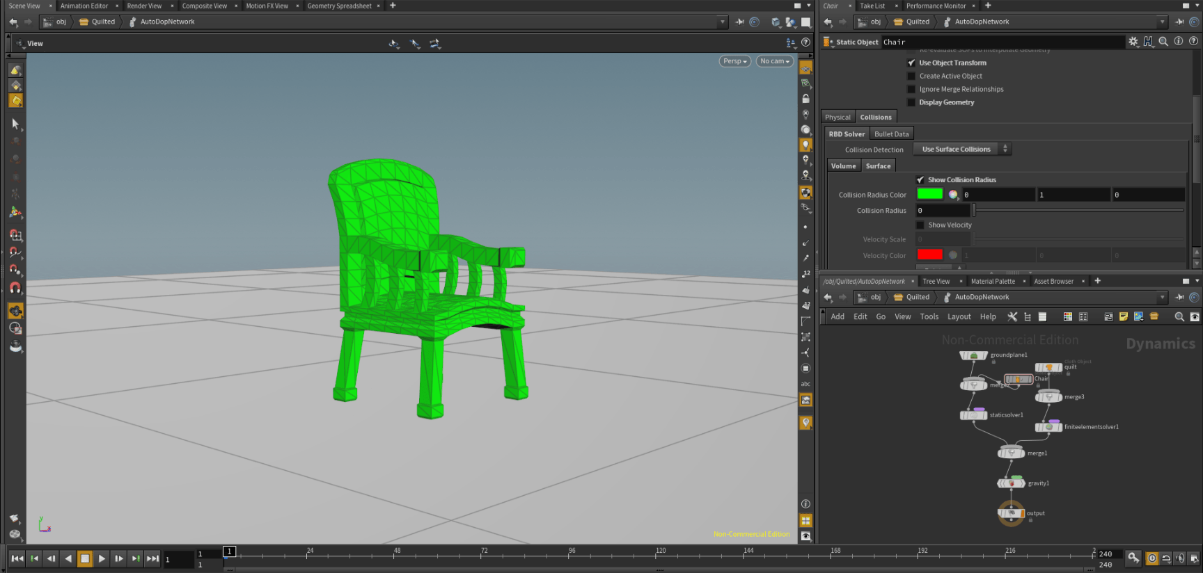
An example of surface collision detection.
Next Steps
- Utilise my knowledge of collisions and particles to produce a few experimental simulations
- Begin to learn about fluids within Houdini